Quick Answer
RAID 6 uses a dual distributed parity scheme, which means it uses two parity blocks per stripe to provide protection against up to two disk failures. The formula for calculating the total capacity of a RAID 6 array is:
Total capacity = (Number of disks – 2) * Size of smallest disk
So for example, in a 6 disk RAID 6 array with four 1TB disks and two 2TB disks, the total capacity would be:
(6 – 2) * 1TB = 4TB
What is RAID?
RAID stands for Redundant Array of Independent Disks. It is a data storage technology that combines multiple disk drive components into a logical unit. Data is distributed across the drives in one of several ways called RAID levels, depending on what level of redundancy and performance is required.
The different RAID levels provide different combinations of increased data reliability and/or increased input/output performance relative to single drives. Some key RAID terms include:
– Mirroring: 100% duplication of data across drives
– Striping: Segmenting data across drives in blocks
– Parity: Calculation of error correction data spread across drives
– Spanning: Concatenation of drives to create a large logical drive
Some common RAID levels include:
– RAID 0: Striping without parity or mirroring. Provides performance but no redundancy.
– RAID 1: Mirroring without parity or striping. Provides redundancy but no performance gain.
– RAID 5: Striping with distributed parity. Provides redundancy and read performance gains.
– RAID 6: Striping with dual distributed parity. Provides redundancy and read performance with up to 2 drive failures.
What is parity and why is it used?
Parity refers to calculated error correction data that is spread across the disks in an array. It provides redundancy which allows data recovery in case of a disk failure.
Here’s a simple example to illustrate how parity works:
Say we have a 3 disk RAID 5 array with disks A, B, and C. The data is striped across the three disks in blocks:
Disk A: 1, 4, 7
Disk B: 2, 5, 8
Disk C: 3, 6, P
The letter P refers to the parity block. It is calculated based on blocks 1-8. If any single disk fails, the missing data can be re-calculated using the parity block.
So if Disk C fails, blocks 3 and 6 can be re-calculated using 1, 2, 4, 5, 7, 8, and P. This provides protection against a single disk failure.
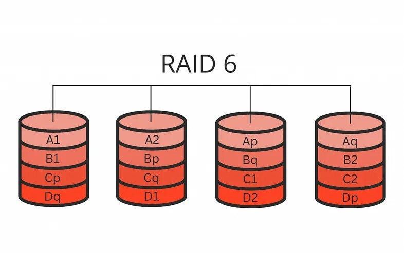
RAID 6 extends this model by using a second distributed parity block (Q). This allows protection against up to two disk failures.
The RAID 6 formula
RAID 6 utilizes block-level striping with double distributed parity. This means data is split into blocks which are striped across multiple drives, with parity calculated and written across two drives.
The formula to calculate the total usable capacity of a RAID 6 array is:
Total capacity = (Number of disks – 2) * Size of smallest disk
Let’s break this down:
– Number of disks – The total number of disks in the array
– Minus 2 – The two disks used for parity
– Multiplied by the size of the smallest disk – To account for unequal disk sizes
For example, consider a RAID 6 array with:
– 6 total disks
– Two 1TB disks
– Four 2TB disks
Plugging this into the formula:
Total capacity = (6 – 2) * 1TB
= 4 * 1TB
= 4TB
The two 2TB disks used for parity are subtracted, so the total usable capacity is equal to the four 1TB data disks.
Why is the formula designed this way?
The RAID 6 formula is designed to account for the overhead of dual parity in the array. By subtracting 2 disks from the total, it reserves those disks for parity data rather than usable capacity.
Using the size of the smallest disk as the multiplier ensures that available capacity is not overestimated if there are disks of different sizes. The smallest disk determines the maximum amount of data that can be safely striped across a parity stripe.
Subtracting the parity disks and using the smallest drive size provides a simple, reliable way to calculate the usable space in a fault tolerant RAID 6 configuration.
Examples
Here are some examples of using the RAID 6 capacity formula with different disk configurations:
4 disks, all 1TB
Total capacity = (4 – 2) * 1TB = 2TB
6 disks, 2 x 1TB and 4 x 2TB
Total capacity = (6 – 2) * 1TB = 4TB
8 disks, 6 x 2TB and 2 x 4TB
Total capacity = (8 – 2) * 2TB = 12TB
12 disks, 8 x 4TB and 4 x 6TB
Total capacity = (12 – 2) * 4TB = 40TB
In each case, the formula takes the total number of disks, subtracts 2 for parity, and multiplies by the size of the smallest disk to determine the usable array capacity.
Accounting for disk failures
An important consideration with RAID 6 is how disk failures impact available capacity.
With single parity RAID 5, the array can tolerate 1 disk failure without data loss. But total capacity is reduced by 1 disk while running in a degraded state until the failed drive is replaced and rebuilt.
RAID 6 can tolerate up to 2 disk failures. But each disk that fails reduces total capacity by 1 disk during rebuild:
– 0 failed disks = Full capacity
– 1 failed disk = Total capacity – 1 disk
– 2 failed disks = Total capacity – 2 disks
So in a 6 disk RAID 6 array, failure of 2 disks would reduce available capacity from 4 disks down to 2 disks during the rebuild process.
RAID 6 rebuild process
When a disk fails in a RAID 6 array, a rebuild process is initiated when a replacement disk is inserted to restore redundancy and full capacity.
The rebuild involves:
1. The replacement disk is inserted and initialized.
2. The parity data is read from the surviving disks.
3. The missing data is calculated from the parity data and written to the replacement disk.
4. Normal redundant operation resumes when rebuild completes.
The larger the disks, the longer the rebuild takes. During this time the array is vulnerable to a second disk failure.
A best practice is to use smaller capacity, higher RPM drives with short rebuild times. Monitoring drive health is also important.
RAID 6 performance
RAID 6 performance characteristics:
– Reads are faster since segment blocks can be read in parallel from multiple disks.
– Writes are slower due to parity calculation overhead.
– More disk I/O is required for writes compared to RAID 5 due to second parity block.
– Rebuild times take longer compared to RAID 5.
In general, RAID 6 provides significantly better read performance than a single disk, but slower write performance. The tradeoff is higher fault tolerance from dual parity.
When to use RAID 6
RAID 6 offers excellent performance and redundancy for scenarios that require high availability and can tolerate slightly slower write speeds. Applications include:
– Transactional databases
– Server applications with mostly read operations
– Media servers streaming large blocks of content
– Archival storage where all data is critical
The dual parity makes RAID 6 ideal for mission critical storage that cannot have downtime or data loss from disk failures. The write penalty is a reasonable tradeoff for highly resilient data storage.
Alternatives to RAID 6
Alternatives to consider instead of RAID 6:
– RAID 10 – Mirroring and striping without parity. Provides performance and redundancy but lower capacity efficiency.
– RAID 60 – Combination of RAID 6 and 0. Stripes data across multiple RAID 6 arrays. Offers strong redundancy with better performance than RAID 6 alone.
– RAID 50 – RAID 5 striped across multiple arrays. Less redundancy than RAID 6 but better write performance.
– Erasure coding – Mathematical function to reconstruct data from fewer parity blocks. Lower overhead than RAID 6 but more complex.
– ZFS – Filesystem with built-in redundancy through mirroring or erasure coding. Filesystem-level rather than block-level.
The alternatives provide different tradeoffs between redundancy, performance, and usable capacity that may be better suited depending on workload and availability requirements.
Software vs hardware RAID 6
RAID 6 can be implemented in software or hardware:
– Software RAID – RAID is managed by the operating system. More flexible and doesn’t require specialized hardware. But consumes CPU resources.
– Hardware RAID – Dedicated RAID controller card manages the array. Offloads processing overhead from main CPU. But less flexible and more expensive.
Software RAID 6 is a good choice for general purpose servers to provide redundancy without expensive hardware controllers. Performance may suffer under heavy workloads.
Hardware RAID 6 delivers better performance under load but requires investing in a high-quality RAID controller. Makes sense for mission critical systems that need fast rebuild times.
RAID 6 with SSDs vs HDDs
Solid state drives (SSDs) and hard disk drives (HDDs) both work with RAID 6, with different considerations:
– SSDs – Faster performance but higher cost per gigabyte. Make sense for smaller arrays focused on speed.
– HDDs – Slower but lower cost. Better suited for high capacity arrays where cost is a factor.
– SSD cache – SSDs can be used as a cache layer to accelerate performance of a HDD RAID 6 array. Provides a hybrid approach.
Because RAID 6 has write performance penalties, SSDs can help mitigate this by providing faster parity calculations and disk access. However SSD endurance may be a concern with constant parity writes.
HDDs allow building much higher capacity RAID 6 arrays cost effectively. But slower rebuild times remain an issue. Combining SSD caching with HDDs offers a balance of performance, capacity, and cost.
Choosing RAID 6 disk types and sizes
When selecting disks for RAID 6, key considerations include:
– Drive interface – Faster interfaces like SAS and NVMe provide better performance.
– Drive RPM – 15k RPM drives rebuild quicker than 7200 RPM models.
– Drive capacity – Larger drives take longer to rebuild. Combining small and large drives can help.
– Number of disks – More disks increase size but reduce performance. 8-12 is a common range.
– Hot spares – Additional standby disks that can automatically rebuild a failed drive.
– Mixing types – Using SSDs for caching can improve HDD array performance.
Carefully benchmarking options and checking manufacturer recommendations can help select optimal drive configurations for a RAID 6 array. Matching drives for consistency is also best practice.
Implementing software RAID 6
Major steps to implement software RAID 6:
1. Assess storage requirements – capacity, performance, availability needs.
2. Select server and drives to meet requirements.
3. Back up existing data if any.
4. Create RAID 6 array via OS tools like mdadm on Linux or Storage Spaces on Windows.
5. Format file system on RAID array to mount volumes.
6. Migrate data to array.
7. Configure monitoring and hot spares for proactive maintenance.
8. Test fault tolerance by simulating drive failures.
Following best practices for drive selection, OS configuration, and ongoing monitoring helps optimize reliability and performance.
Example software RAID 6 setup
Here is an example RAID 6 setup on Ubuntu Linux using mdadm:
1. Install 4 x 2TB HDDs in server.
2. Back up existing data.
3. Use mdadm to create RAID 6 array:
“`bash
sudo mdadm –create /dev/md0 –level=6 –raid-devices=4 /dev/sdb /dev/sdc /dev/sdd /dev/sde
“`
4. Format XFS filesystem on /dev/md0.
5. Mount array under /data.
6. Add monitoring with mdadm and install hot spares.
7. Test failures by marking drives as failed.
8. Rebuild drives by adding back to array.
This creates a 4 x 2TB RAID 6 array for 8TB total capacity. We can monitor and simulate drive failures to validate redundancy.
Hardware RAID 6 configuration
To configure RAID 6 with a hardware RAID controller:
1. Install RAID controller card in server.
2. Connect drives to controller ports.
3. Boot into controller interface (Ctrl-R, F2 etc).
4. Select drives and create new RAID 6 array.
5. Configure array properties like stripe size.
6. Initialize and format array.
7. View and manage array via controller software.
8. Install monitoring software to track drive health.
Hardware RAID 6 setup is largely managed through the vendor controller interface rather than the OS. But OS tools can provide additional monitoring and alerts.
Monitoring RAID 6 arrays
It is critical to monitor RAID 6 arrays for drive failures and rebuild status. Key items to track:
– Drive errors – Scan logs for drive failure alerts.
– SMART stats – Review drive SMART data for signs of impending failure.
– Rebuild status – Monitor percent completed when rebuilding a failed drive.
– Performance stats – Watch for slowdowns indicating problems.
– Array sync status – Ensure synchronization between disk writes.
– Spare drive capacity – Be alerted when hot spare space is getting low.
Monitoring tools like mdadm for Linux or Storage Spaces in Windows provide notifications when drives fail or arrays become degraded. Third party tools also available.
Automated monitoring and alerts help detect and resolve RAID issues quickly.
Managing hot spares
Hot spare drives are standby disks that can automatically rebuild arrays when a failure occurs. To manage them effectively:
– Use enterprise-grade hot swap drives for reliability.
– Ensure spares have adequate capacity for the largest drive in the array.
– Allow OS/controller to identify and designate spare drives.
– Place spares in empty slots with access to array controller.
– Test rebuilding with spares by simulating drive failures.
– Replace used spares immediately so spare capacity is always available.
– Monitor spare availability and capacity as part of array monitoring.
Properly configured hot spares can greatly reduce rebuild times and lower the risk of a second drive failure during rebuild.
Recovering from failed RAID 6 arrays
If too many disk failures occur in a RAID 6 array, it can become critically damaged and unusable. Recovery options include:
– Replace failed drives – If at least 4 drives are still operational in a 6 disk array, replace failed drives to recover.
– Rebuild from parity – If parity blocks are still available, recovery may be possible. Requires RAID recovery software.
– Restore from backup – A current backup allows restoring data if the array cannot be rebuilt.
– Professional data recovery – Data recovery firms may be able to recover portions of data at high cost.
– Start over – In extreme cases, the only option may be to create a new array from scratch and reload data.
RAID 6 offers excellent redundancy, but it is not infallible. Regular backups, hot spares, and RAID monitoring provide the best chance of recovering from severe failures.
Conclusion
The formula for RAID 6 capacity calculates usable space by accounting for the overhead of dual parity. Subtracting two disks for parity and multiplying by the smallest disk size provides an accurate estimate of total capacity.
RAID 6 provides highly reliable storage using dual parity at the cost of reduced write performance. Careful monitoring, hot spares, proper drive selection, and backups are key to maximizing availability and recovering from failures.
Understanding the core RAID 6 formula, strengths, tradeoffs, and recovery techniques allows properly architecting arrays to meet performance, capacity, and availability goals.
